Discovering Spatial Ecotypes from a Single Spatial Transcriptomics Sample
Source:vignettes/SingleSample.Rmd
SingleSample.RmdOverview
In this tutorial, we will illustrate how to perform de novo discovery of spatial ecotypes from a single-cell spatial transcriptomics (ST) dataset using SpatialEcoTyper.
Input requirement
All single-cell-scale ST datasets can be analyzed with SpatialEcoTyper to discover spatial ecotypes (SEs). In our study (Zhang et al., Nature), we applied SpatialEcoTyper to both MERSCOPE and Xenium datasets and identified highly consistent pan-cancer spatial ecotypes across the two platforms.
Single-cell ST gene expression profiles are inherently affected by transcript spillover. In our study, we addressed this issue by constructing a whitelist of genes expressed in each cell type using a pan-cancer scRNA-seq atlas and removing transcripts that were not included in the corresponding cell-type whitelist. Alternatively, computational methods such as SPLIT have been developed to decontaminate single-cell ST data by correcting transcript spillover. We recommend applying either a whitelist-based filtering strategy or a dedicated decontamination method before running SpatialEcoTyper, as improving data quality can substantially enhance the robustness and biological interpretability of the discovered spatial ecotypes.
The SpatialEcoTyper requires two input data objects:
- Gene expression matrix: a numeric matrix with genes as rows and cells as columns.
- Metadata: a data frame containing at least three columns: “X” (x-coordinate), “Y” (y-coordinate), and “CellType” (cell type annotation). Row names must match the column names (cell IDs) in the expression matrix.
Example data
We will be analyzing single-cell spatial transcriptomics data from a melanoma sample (raw data available in Vizgen’s MERSCOPE FFPE Human Immuno-oncology). This demo data comprises the spatial expression of 500 genes across 27,907 cells, which are categorized into ten distinct cell types: B cells, CD4 T cells, CD8 T cells, NK cells, plasma cells, macrophages, dendritic cells (DC), fibroblasts, endothelial cells, and melanoma cells. For this tutorial, melanoma cells are excluded to reduce computational time; in practice, any cell types can be included.
All cells in this demo data are grouped into tumor (tumor and inner margin) and stroma regions (stroma and outer margin) based on the density of cancer cells, as described in the CytoSPACE paper. The inner and outer margins are defined as regions extending 250 μm inside and outside the tumor boundaries, respectively. Furthermore, we quantified each cell’s distance to the tumor–stroma interface by calculating the shortest Euclidean distance to the nearest tumor region (for stromal cells) or stromal region (for tumor cells). A positive distance indicates cells located within the tumor region, while a negative distance indicates cells located within the stroma.
First load required packages for this vignette
suppressPackageStartupMessages(library(dplyr))
suppressPackageStartupMessages(library(ggplot2))
suppressPackageStartupMessages(library(parallel))
suppressPackageStartupMessages(library(Seurat))
suppressPackageStartupMessages(library(data.table))
suppressPackageStartupMessages(library(R.utils))

library(SpatialEcoTyper)
Quick start
## Load single-cell gene expression matrix (genes × cells)
url <- "https://spatialecotyper.stanford.edu/inc/inc.public.vignettes.php?file=Melanoma1_subset_counts.tsv.gz"
scdata <- fread(url, sep = "\t",header = TRUE, data.table = FALSE)
rownames(scdata) <- scdata[, 1]
scdata <- as.matrix(scdata[, -1])

## Normalize the gene expression data
normdata <- NormalizeData(scdata)

## Load single-cell metadata
## Required columns: "X", "Y", and "CellType"
## Row names must match the cell IDs in the expression matrix
url <- "https://spatialecotyper.stanford.edu/inc/inc.public.vignettes.php?file=Melanoma1_subset_scmeta.tsv"
scmeta <- read.table(url, sep = "\t", header = TRUE, row.names = 1)
scmeta <- scmeta[match(colnames(scdata), rownames(scmeta)), ]
head(scmeta[, c("X", "Y", "CellType")])

## Discover spatial ecotypes using the SpatialEcoTyper
se_results <- SpatialEcoTyper(normdata, scmeta,
                              outprefix = "Melanoma1_subset",
                              nfeatures = 300, radius = 50, ncores = 2)
Loading data
Text files as input
Large text files can be loaded into R using the fread
function from the data.table package.
## Load single-cell gene expression matrix (genes × cells)
url <- "https://spatialecotyper.stanford.edu/inc/inc.public.vignettes.php?file=Melanoma1_subset_counts.tsv.gz"
scdata <- fread(url, sep = "\t",header = TRUE, data.table = FALSE)
rownames(scdata) <- scdata[, 1]
scdata <- as.matrix(scdata[, -1])
head(scdata[, 1:5])
## HumanMelanomaPatient1__cell_3655 HumanMelanomaPatient1__cell_3657
## PDK4 0 1
## TNFRSF17 0 0
## ICAM3 0 0
## FAP 1 0
## GZMB 0 0
## TSC2 0 0
## HumanMelanomaPatient1__cell_3658 HumanMelanomaPatient1__cell_3660
## PDK4 1 0
## TNFRSF17 0 0
## ICAM3 0 0
## FAP 0 0
## GZMB 0 0
## TSC2 0 0
## HumanMelanomaPatient1__cell_3661
## PDK4 0
## TNFRSF17 0
## ICAM3 0
## FAP 0
## GZMB 0
## TSC2 0
## Load single-cell metadata
## Required columns: "X", "Y", and "CellType"
## Row names must match the cell IDs in the expression matrix
url <- "https://spatialecotyper.stanford.edu/inc/inc.public.vignettes.php?file=Melanoma1_subset_scmeta.tsv"
scmeta <- read.table(url, sep = "\t", header = TRUE, row.names = 1)
scmeta <- scmeta[match(colnames(scdata), rownames(scmeta)), ]
head(scmeta[, c("X", "Y", "CellType")])
## X Y CellType
## HumanMelanomaPatient1__cell_3655 1894.706 -6367.766 Fibroblast
## HumanMelanomaPatient1__cell_3657 1942.480 -6369.602 Fibroblast
## HumanMelanomaPatient1__cell_3658 1963.007 -6374.026 Fibroblast
## HumanMelanomaPatient1__cell_3660 1981.600 -6372.266 Fibroblast
## HumanMelanomaPatient1__cell_3661 1742.939 -6374.851 Fibroblast
## HumanMelanomaPatient1__cell_3663 1921.683 -6383.309 FibroblastSparse matrix as input
SpatialEcoTyper
supports sparse matrix as input. Mtx files can be loaded into R using
the ReadMtx
function from the Seurat package.
scdata <- ReadMtx(mtx = "https://spatialecotyper.stanford.edu/inc/inc.public.vignettes.php?file=Melanoma1_subset_counts.mtx.gz",
                  cells = "https://spatialecotyper.stanford.edu/inc/inc.public.vignettes.php?file=Melanoma1_subset_cells.tsv.gz",
                  features = "https://spatialecotyper.stanford.edu/inc/inc.public.vignettes.php?file=Melanoma1_subset_genes.tsv.gz",
                  feature.column = 1, cell.column = 1)
Data normalization
Gene expression data should be normalized prior to SpatialEcoTyper analysis. The data can be performed using either NormalizeData or SCTransform.
Here, we are normalizing using NormalizeData.
normdata <- NormalizeData(scdata)Using SCTransform for the normalization:
For SCTransform normalization, we recommend installing
the glmGamPoi package to accelerate computation.
if(!"glmGamPoi" %in% rownames(installed.packages())){
  BiocManager::install("glmGamPoi")
}
tmpobj <- CreateSeuratObject(scdata) %>%
      SCTransform(clip.range = c(-10, 10), verbose = FALSE)

seurat_version = as.integer(gsub("\\..*", "", as.character(packageVersion("SeuratObject"))))
if(seurat_version<5){
  normdata <- GetAssayData(tmpobj, "data")
}else{
  normdata <- tmpobj[["SCT"]]$data
}
Preview of the sample
The SpatialView function can be used to visualize single cells within the tissue. You can color the cells by cell type or predefined spatial regions.
# Visualize the cell type annotations in the tissue
SpatialView(scmeta, by = "CellType") + scale_color_manual(values = pals::cols25())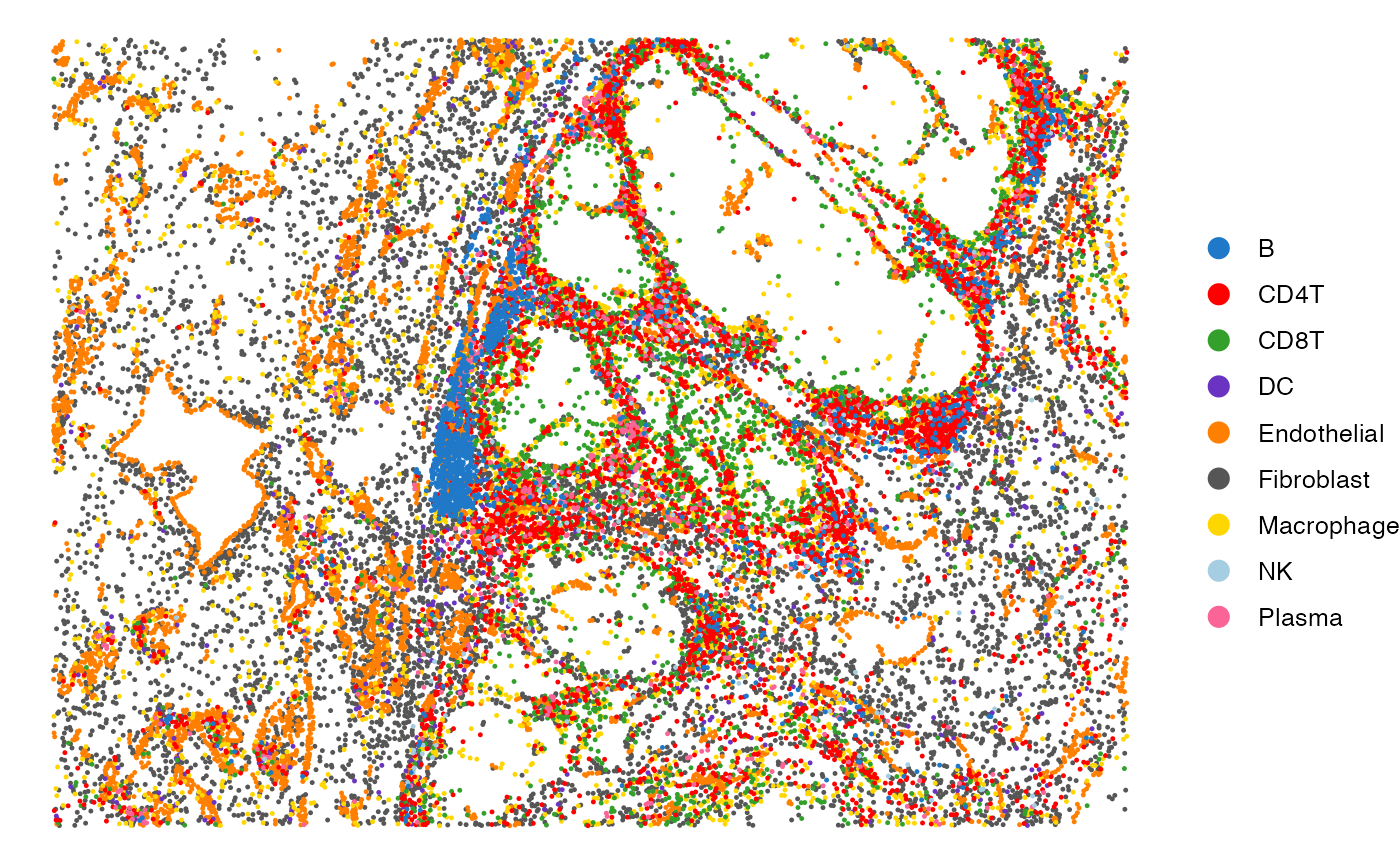
# Visualize the regions in the tissue
SpatialView(scmeta, by = "Region") + scale_color_brewer(type = "qual", palette = "Set1")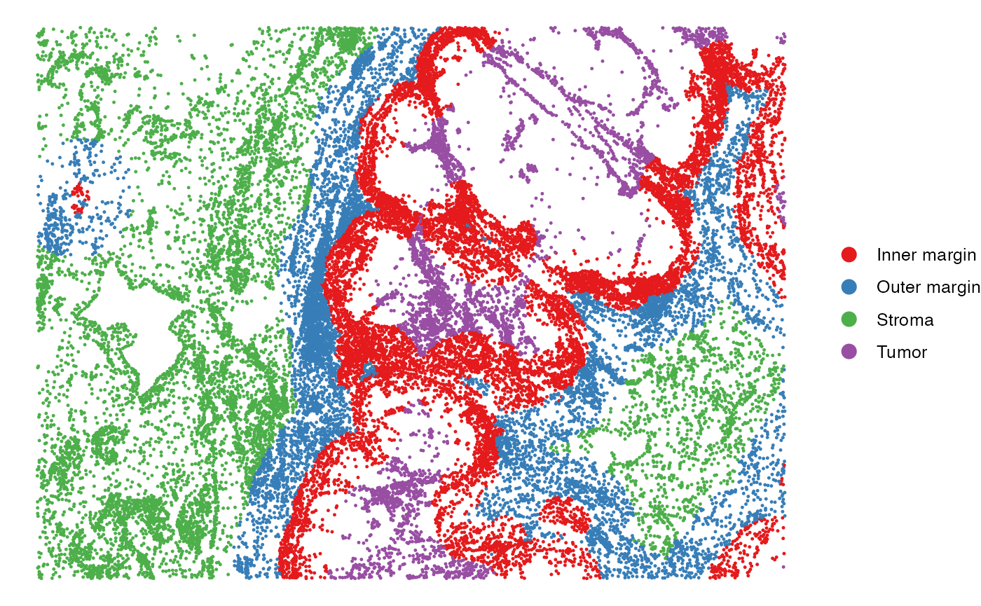
The SpatialView function can also be used to visualize continuous characteristics, such as the minimum distance of each single cell to tumor/stroma margin. Here, positive distances indicate cells located within the tumor region, while negative distances denote cells within the stroma.
# Visualize the distance to tumor margin
SpatialView(scmeta, by = "Dist2Interface") +
  scale_colour_gradient2(low = "#5e3c99", high = "#e66101",
                         mid = "#d9d9d9", midpoint = 0) +
  labs(color = "Distance to\ntumor margin")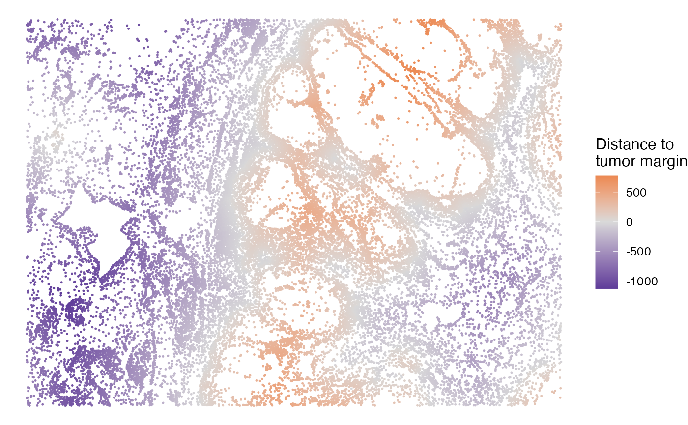
SE discovery using SpatialEcoTyper
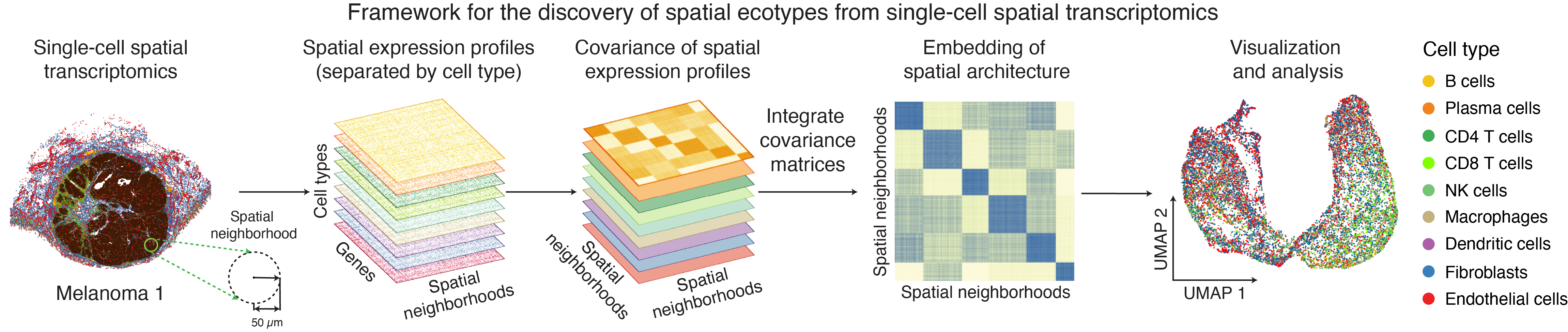
The SpatialEcoTyper function is designed to identify spatial ecotypes (SEs) from single-cell spatial transcriptomics data. The workflow begins by defining spatial neighborhoods (SNs) on a regular grid and constructing cell type–specific gene expression profiles (GEPs) for each SN. For each cell type, a similarity network is constructed, where nodes represent SNs and edges reflect transcriptional similarity. These cell type–specific networks are then integrated using Similarity Network Fusion (SNF), originally developed for multi-omics data integration (Wang et al., 2014). This yields a fused similarity network that captures shared spatial transcriptomic variation across cell types, enabling the identification of SEs through clustering. Before start, please check key arguments here.
Selection of Spatial EcoTyper parameters
Choosing the radius parameter: The optimal spatial
neighborhood radius depends on the biological question.
Larger radii capture broader regional patterns, whereas smaller radii
resolve more localized cellular niches. In our analysis, we used a
radius of 50 µm, which typically includes ~10–80 neighboring cells and
provides a practical balance between granularity and robustness.
Choosing the number of variable features: The
nfeatures argument should be selected according to the
underlying data platform. For Vizgen MERSCOPE V1 (500-gene panel) and
Xenium Prime data, we used 200/300 highly variable features. As
single-cell spatial transcriptomics technologies continue to evolve, the
number of detectable genes per cell has steadily increased. For example,
the 10x Atera captures over 1,000 genes per cell on average. For such
high-complexity datasets, we recommend using up to 1,000 highly variable
genes for downstream analysis to better capture biological
variability.
Limiting the number of cell types per spatial
neighborhood: The min.cts.per.region argument
allows users to filter spatial regions based on cellular diversity by
requiring a minimum number of distinct cell types per region (default: ≥
2). This helps ensure that downstream analyses focus on biologically
informative neighborhoods with sufficient cellular heterogeneity.
filter.region.by.celltypes
argument allows users to define a set of cell types of interest. When
specified, only spatial regions that contain all of the selected cell
types are retained for downstream analysis. This enables focused
interrogation of neighborhoods enriched for predefined cellular
compositions, facilitating the identification of multicellular
ecosystems associated with the target cell types.
se_results <- SpatialEcoTyper(normdata, scmeta,
                              outprefix = "Melanoma1_subset",
                              nfeatures = 300, radius = 50, ncores = 2)
Optimizing memory usage
The similarity network fusion (Step 2 of SpatialEcoTyper) is the most computationally demanding step and its runtime increases with the number of spatial neighborhoods (SNs) per sample. Performance depends on dataset size and structure rather than tissue technology.
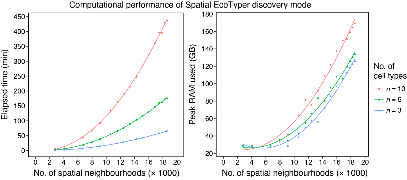 For example, an analysis involving 10 cell types and 18,564 SNs required
436 minutes of runtime and reached a peak memory usage of 169 GB. This
benchmark was obtained on a computing cluster equipped with an AMD EPYC
7543 processor (2.75 GHz) and 256 GB RAM, using a single CPU core and
excluding data loading time.
For example, an analysis involving 10 cell types and 18,564 SNs required
436 minutes of runtime and reached a peak memory usage of 169 GB. This
benchmark was obtained on a computing cluster equipped with an AMD EPYC
7543 processor (2.75 GHz) and 256 GB RAM, using a single CPU core and
excluding data loading time.
To reduce runtime, users can increase the number of cores via the
ncores parameter. However, this parallelization comes at
the cost of increased memory consumption.
When memory resources are limited, users can increase the
grid.size parameter, which will reduce the number of
spatial neighborhoods, thereby substantially lowering memory usage and
improving computational efficiency.
SpatialEcoTyper result
When the outprefix is specified, the SpatialEcoTyper result will
be saved as a RDS file named
outprefix_SpatialEcoTyper_results.rds. The result can be
loaded into R using readRDS.
se_results <- readRDS("Melanoma1_subset_SpatialEcoTyper_results.rds")The SpatialEcoTyper result is a list containing two key components:
- Seurat object constructed from the fused network embedding of spatial neighborhoods, enabling clustering and downstream visualization of SEs.
- Metadata, single-cell metadata with SE annotations appended.
# Extract the Seurat object and updated single-cell metadata
obj <- se_results$obj # A Seurat object
scmeta <- se_results$metadata # Single-cell meta data, with SE annotation added
head(scmeta)
## X Y CellType CellTypeName
## HumanMelanomaPatient1__cell_3655 1894.706 -6367.766 Fibroblast Fibroblasts
## HumanMelanomaPatient1__cell_3657 1942.480 -6369.602 Fibroblast Fibroblasts
## HumanMelanomaPatient1__cell_3658 1963.007 -6374.026 Fibroblast Fibroblasts
## HumanMelanomaPatient1__cell_3660 1981.600 -6372.266 Fibroblast Fibroblasts
## HumanMelanomaPatient1__cell_3661 1742.939 -6374.851 Fibroblast Fibroblasts
## HumanMelanomaPatient1__cell_3663 1921.683 -6383.309 Fibroblast Fibroblasts
## Region Dist2Interface SE
## HumanMelanomaPatient1__cell_3655 Stroma -883.1752 NewSE5
## HumanMelanomaPatient1__cell_3657 Stroma -894.8463 NewSE8
## HumanMelanomaPatient1__cell_3658 Stroma -904.1115 NewSE8
## HumanMelanomaPatient1__cell_3660 Stroma -907.8909 NewSE8
## HumanMelanomaPatient1__cell_3661 Stroma -874.2712 NewSE1
## HumanMelanomaPatient1__cell_3663 Stroma -903.6559 NewSE5
table(scmeta$SE) ## The number of cells in each SE##
## NewSE1 NewSE2 NewSE3 NewSE4 NewSE5 NewSE6 NewSE7 NewSE8
## 2952 3320 7006 4772 3077 1216 3344 1715Note: SpatialEcoTyper applies stringent quality
control to exclude low-quality spatial neighborhoods, including those
with insufficient detected genes (min.features), too few
cells (min.cells), or insufficient cell type diversity
(min.cts.per.region). These regions are labeled as NA.
Regions excluded at one resolution (radius,
grid.size) may be retained at a lower resolution if they
pass QC. In practice, different resolutions have minimal impact on
overall results. By default, NA regions are removed. To retain all
cells, set dropcell = FALSE.
Embedding of spatial architecture
The embedding of spatial neighborhoods can be visualized using
standard Seurat
functions such as DimPlot and FeaturePlot.
These visualizations help to explore the spatial organization and
heterogeneity within the tissue.
Note: The embedding and clustering results differ slightly between Seurat v4 and v5. However, the overall clustering patterns remain largely consistent, with an Adjusted Rand Index (ARI) of 0.7 for the demonstration dataset. This consistency ensures that, despite minor variations, the key biological insights are preserved across versions.
Visualizing tumor/stroma regions in the embedding
DimPlot(obj, group.by = "Region") + scale_color_brewer(type = "qual", palette = "Set1")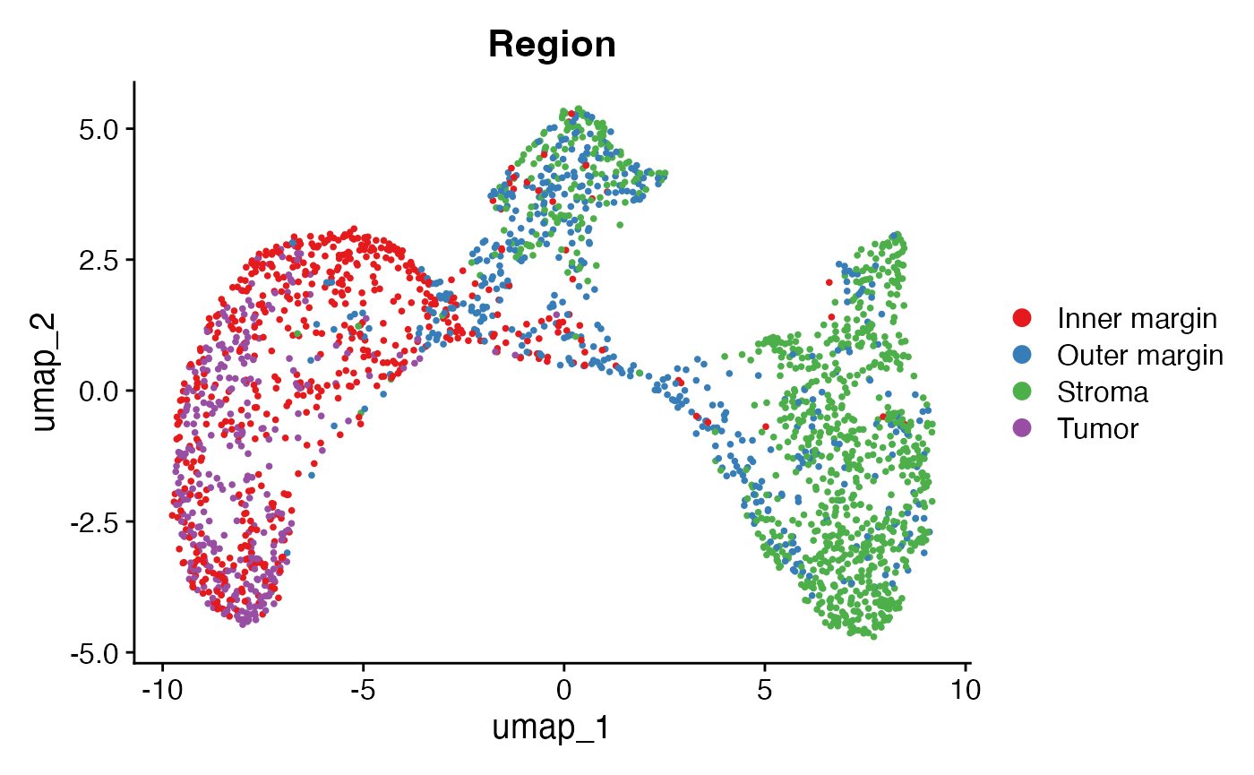
Visualizing the distance of SNs to tumor/stroma interface
This plot shows the distance of each SN to the tumor/stroma interface. Here, positive distances indicate SNs located within the tumor region, while negative distances denote SNs within the stroma.
FeaturePlot(obj, "Dist2Interface", min.cutoff = -600, max.cutoff = 600) +
  scale_colour_gradient2(low = "#5e3c99", high = "#e66101", mid = "#d9d9d9", midpoint = 0)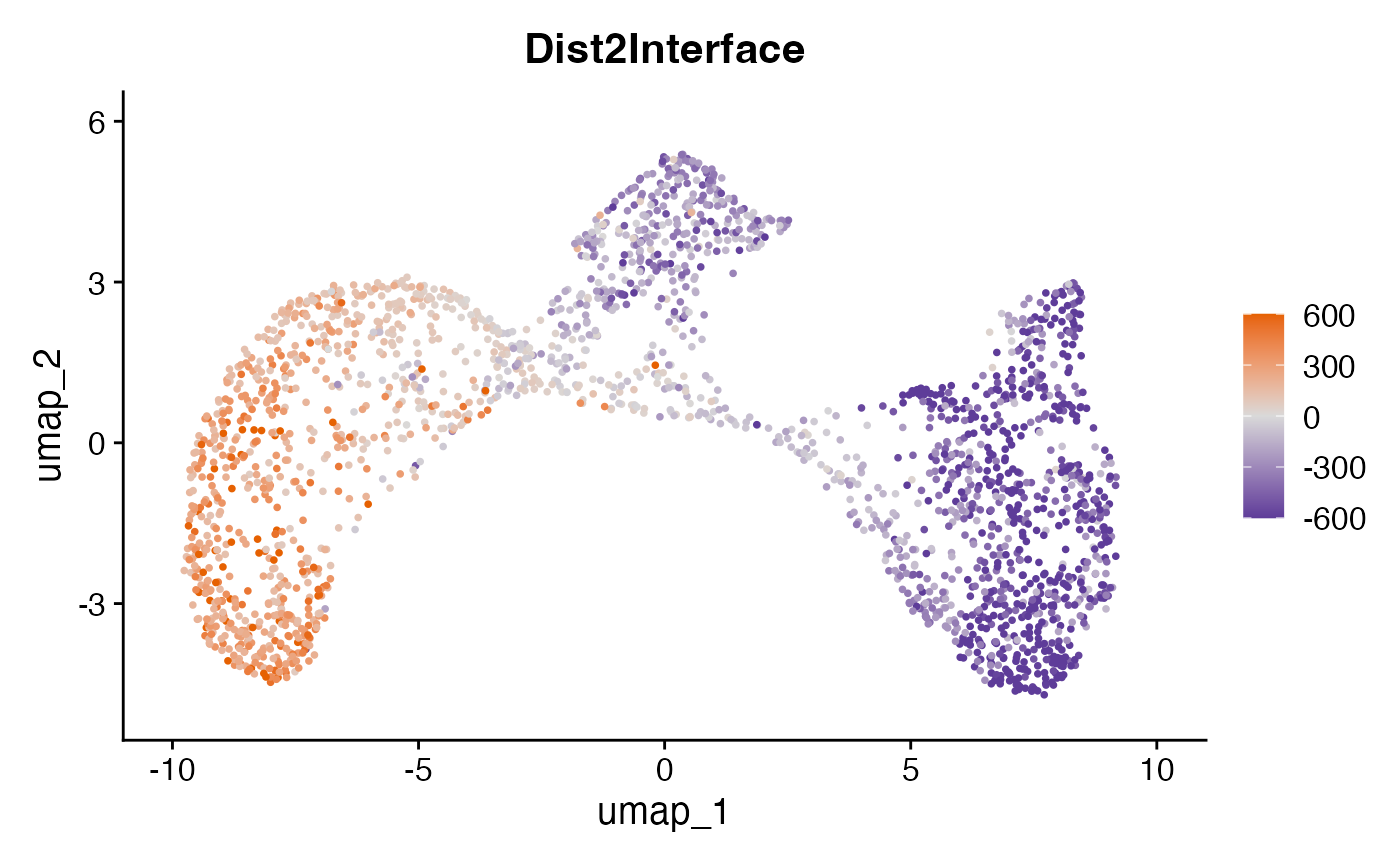
Visualizing spatial ecotypes in the embedding
This plot visualizes the SEs within the spatial embedding. Each SE represents a distinct spatial ecosystem with unique molecular and spatial characteristics, and may also differ in cell type composition.
DimPlot(obj, group.by = "SE") + scale_color_manual(values = pals::kelly()[-1])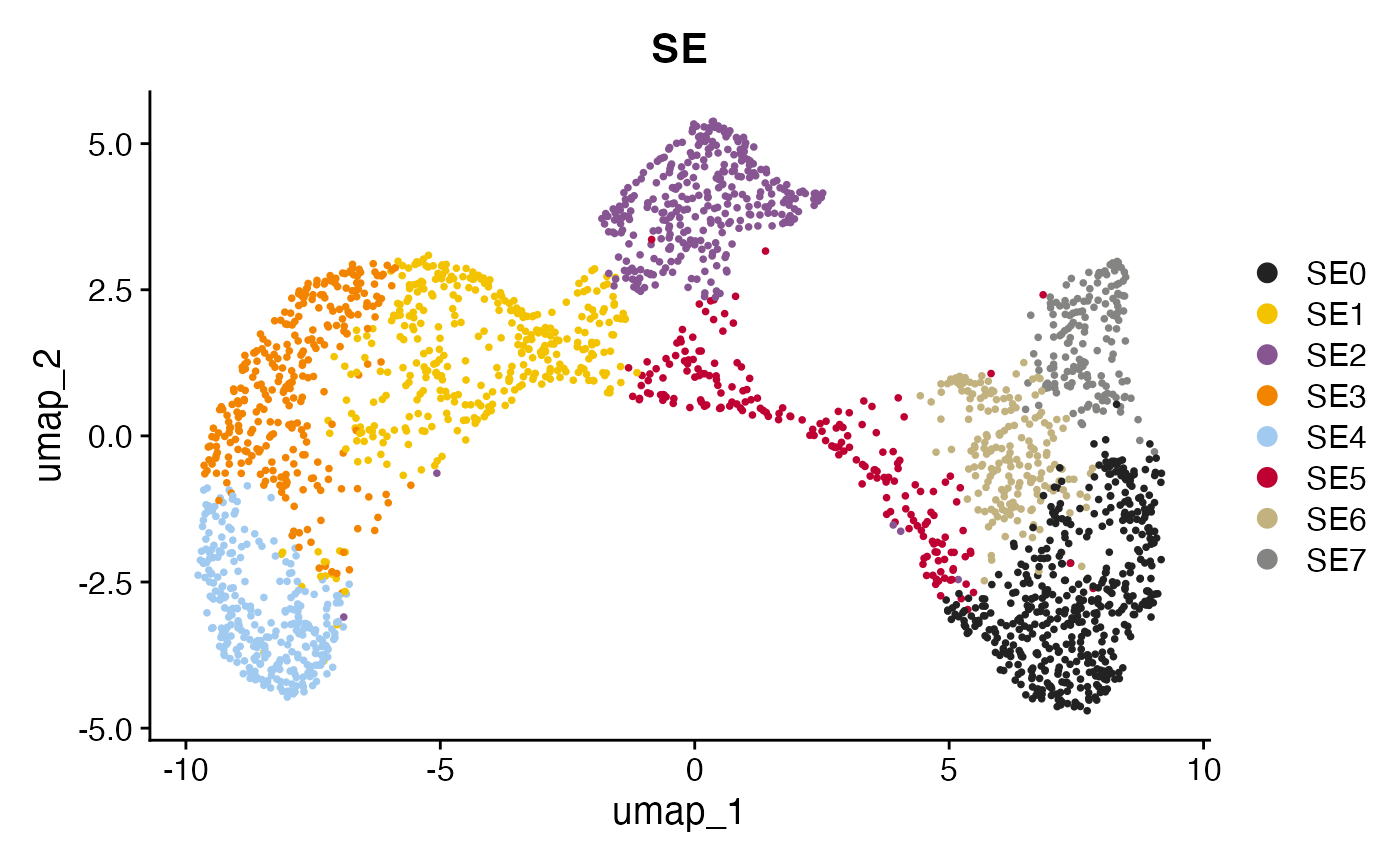
SE characteristics
Visualizing SEs in the tissue
The spatial distribution of SEs within the tissue can be visualized using the SpatialView function.
SpatialView(scmeta, by = "SE")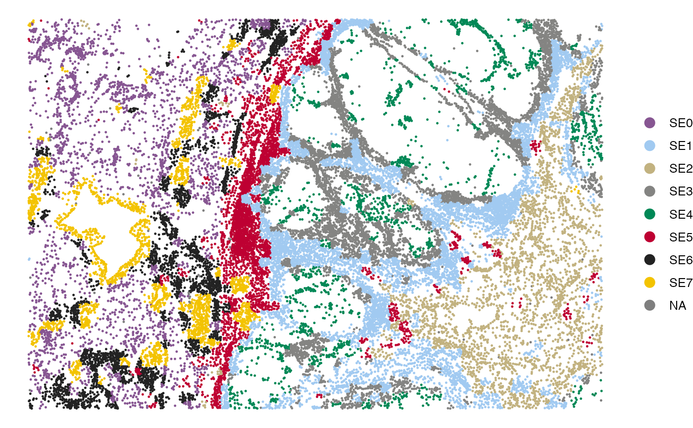
Visualizing the cell type composition of SEs
The bar plot below illustrates the cell type composition within each SE.
gg <- scmeta %>% filter(!is.na(SE)) %>% count(SE, CellType)
ggplot(gg, aes(SE, n, fill = CellType)) +
  geom_bar(stat = "identity", position = "fill") +
  scale_fill_manual(values = pals::cols25()) +
  theme_bw(base_size = 14) + coord_flip() +
  labs(y = "Cell type abundance")
Visualizing the association between SEs and pre-annotated regions
This bar plot shows the enrichment of SEs in pre-defined regions (e.g., tumor and stroma).
gg <- scmeta %>% filter(!is.na(SE)) %>% count(SE, Region)
ggplot(gg, aes(SE, n, fill = Region)) +
  geom_bar(stat = "identity", position = "fill") +
  scale_fill_brewer(type = "qual", palette = "Set1") +
  theme_bw(base_size = 14) + coord_flip() +
  labs(y = "Fraction")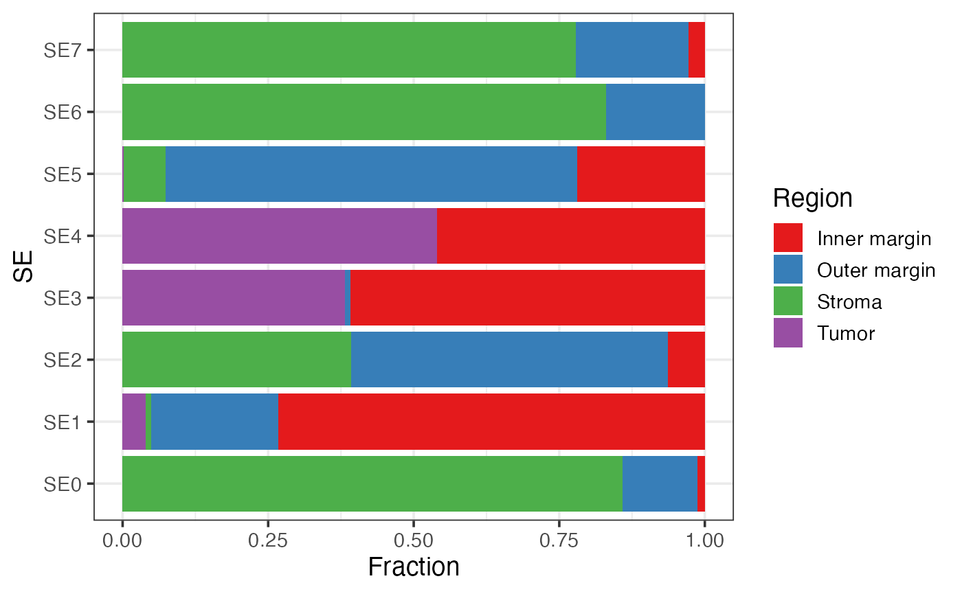
Visualizing the distance of SEs to tumor/stroma interface
This box plot visualizes the distribution of distances of SEs to the tumor/stroma interface. Positive distances indicate cells located within the tumor region, while negative distances denote cells within the stroma. The SEs are ordered by their median distance, highlighting their spatial localization relative to the tumor/stroma interface.
gg <- scmeta %>% filter(!is.na(SE))
## Order SEs by their distance to tumor/stroma interface
tmp <-  gg %>% group_by(SE) %>% summarise(Mid = median(Dist2Interface)) %>% arrange(Mid) %>% pull(SE)
gg$SE = factor(gg$SE, levels = tmp)
ggplot(gg, aes(SE, Dist2Interface)) +
  geom_boxplot() + theme_bw() + labs(y = "Distance to tumor/stroma interface (μm)")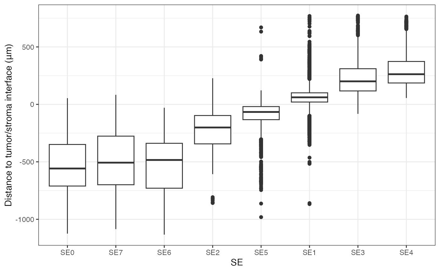
Identification of cell-type-specific SE markers
Differential expression analysis
To identify cell-type-specific SE markers, differential expression
analysis can be performed using the presto
package package. The script below demonstrates how to identify
SE-specific markers within each cell type.
if(!"presto" %in% installed.packages()){
  BiocManager::install("devtools")
  devtools::install_github("immunogenomics/presto")
}
library("presto")

# Ensure normalized data is aligned with metadata
normdata = normdata[, rownames(scmeta)]

# Perform differential expression analysis
degs = lapply(unique(scmeta$CellType), function(ct){
  idx = which(scmeta$CellType==ct & !is.na(scmeta$SE))
  degs = wilcoxauc(normdata[, idx], scmeta$SE[idx])
  degs$CellType = ct
  degs
})
degs = do.call(rbind, degs)

# Example: top markers for CD4 T cells
degs %>% filter(CellType=="CD4T") %>%
  filter(logFC>0 & padj<0.05) %>%
  arrange(desc(logFC)) %>% head()
## feature group avgExpr logFC statistic auc pval
## 1 CTNNB1 NewSE6 1.4430236 0.7282956 222619.0 0.8033539 1.099665e-18
## 2 FOS NewSE7 1.9681507 0.7117793 1289787.0 0.7165499 4.195123e-55
## 3 FN1 NewSE2 1.8704914 0.7071840 876265.5 0.6689581 4.663829e-26
## 4 PKM NewSE6 2.4066543 0.6276660 217859.0 0.7861767 6.478136e-16
## 5 FOXP3 NewSE8 0.9651999 0.6073174 61573.5 0.7011170 1.113723e-04
## 6 CDK2 NewSE6 0.7398827 0.5866178 202262.5 0.7298944 1.772995e-20
## padj pct_in pct_out CellType
## 1 2.265311e-16 92.53731 68.23017 CD4T
## 2 1.728391e-52 96.28099 78.94595 CD4T
## 3 9.607489e-24 84.66077 64.54451 CD4T
## 4 8.896640e-14 100.00000 97.31625 CD4T
## 5 1.529513e-02 61.90476 31.58776 CD4T
## 6 7.304738e-18 58.20896 19.48743 CD4TVisualizing the expression of cell state markers
Once candidate markers are identified, their expression can be visualized across SEs.
Visualizing SE-specific markers using heatmap
The example below identifies SE-specific markers in CD4 T cells and visualizes their relative expression across SEs using a heatmap.
library(tidyr)
# Identify significant DEGs
sigDegs = degs %>% filter(CellType=="CD4T") %>% filter(logFC>0 & padj<0.05)
# Identify genes with highest specificity per SE
top_markers <- sigDegs %>% group_by(feature) %>% arrange(desc(logFC)) %>%
  summarize(Highest_SE = first(group), Highest_logFC = first(logFC),
            Second_logFC = nth(logFC, 2, default = 0),
            Delta = Highest_logFC - Second_logFC) %>% ungroup() %>%
  # Keep top 5 markers per SE based on Delta
  group_by(Highest_SE) %>% arrange(desc(Delta)) %>%
  slice_head(n = 5) %>% ungroup()

# Prepare logFC matrix for heatmap
lfcs = degs %>% filter(CellType=="CD4T") %>%
        pivot_wider(id_cols = feature, names_from = group,
                    values_from = logFC) %>% as.data.frame
rownames(lfcs) = lfcs$feature
lfcs = lfcs[, -1]
gg <- lfcs[top_markers$feature, unique(top_markers$Highest_SE), drop = FALSE]

# Scale for visualization
gg = scale(t(scale(t(gg), center = FALSE)))
# Plot heatmap
HeatmapView(gg, breaks = c(0, 1, 1.5))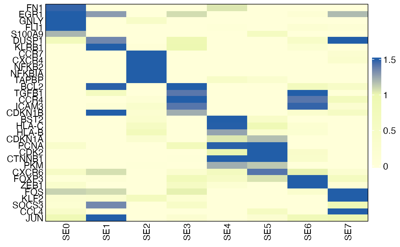
Visualizing an individual marker using box plot
You can also visualize the expression of an individual gene across SEs.
# Subset CD4 T cells with SE annotation
idx = which(scmeta$CellType=="CD4T" & !is.na(scmeta$SE))
gg = scmeta[idx, ]
gg$Expression = normdata["FOXP3", idx]
ggplot(gg, aes(SE, Expression)) + geom_boxplot(outlier.shape = NA) +
  theme_classic(base_size = 14) + ylab("FOXP3 expression")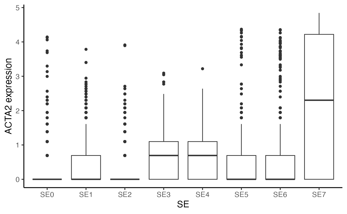
Visualizing expression of SE marker in the tissue
You can also visualize the expression of an individual marker (e.g., FOXP3) or average expression of SE-specific markers in the tissue.
# Visualize gene expression in tissue
gg <- scmeta
gg$Expression = normdata["FOXP3", ]

SpatialView(gg, by = "Expression") +
  scale_color_viridis_c() +
  labs(color = "FOXP3\nexpression")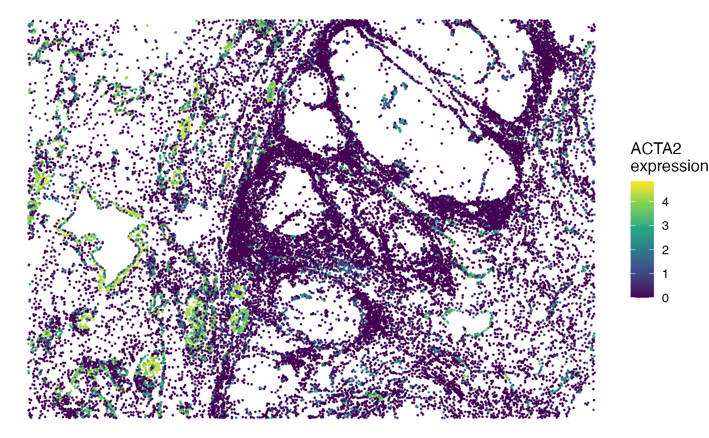
Session info
The session info allows users to replicate the exact environment and identify potential discrepancies in package versions or configurations that might be causing problems.
## R version 4.4.1 (2024-06-14)
## Platform: aarch64-apple-darwin20
## Running under: macOS 26.5.1
##
## Matrix products: default
## BLAS:   /Library/Frameworks/R.framework/Versions/4.4-arm64/Resources/lib/libRblas.0.dylib
## LAPACK: /Library/Frameworks/R.framework/Versions/4.4-arm64/Resources/lib/libRlapack.dylib;  LAPACK version 3.12.0
##
## locale:
## [1] en_US.UTF-8/en_US.UTF-8/en_US.UTF-8/C/en_US.UTF-8/en_US.UTF-8
##
## time zone: America/Los_Angeles
## tzcode source: internal
##
## attached base packages:
## [1] parallel  stats     graphics  grDevices utils     datasets  methods
## [8] base
##
## other attached packages:
##  [1] tidyr_1.3.1           presto_1.0.0          Rcpp_1.1.2
##  [4] SpatialEcoTyper_1.0.4 pals_1.9              NMF_0.28
##  [7] Biobase_2.64.0        BiocGenerics_0.50.0   cluster_2.1.6
## [10] rngtools_1.5.2        registry_0.5-1        RANN_2.6.2
## [13] Matrix_1.7-0          R.utils_2.12.3        R.oo_1.26.0
## [16] R.methodsS3_1.8.2     data.table_1.18.4     Seurat_5.1.0
## [19] SeuratObject_5.0.2    sp_2.1-4              ggplot2_4.0.3
## [22] dplyr_1.2.1
##
## loaded via a namespace (and not attached):
##   [1] RcppAnnoy_0.0.22            splines_4.4.1
##   [3] later_1.3.2                 tibble_3.3.1
##   [5] polyclip_1.10-7             fastDummies_1.7.4
##   [7] lifecycle_1.0.5             sf_1.1-0
##   [9] doParallel_1.0.17           globals_0.16.3
##  [11] lattice_0.22-6              MASS_7.3-60.2
##  [13] magrittr_2.0.5              plotly_4.10.4
##  [15] sass_0.4.9                  rmarkdown_2.28
##  [17] jquerylib_0.1.4             yaml_2.3.10
##  [19] httpuv_1.6.15               glmGamPoi_1.16.0
##  [21] sctransform_0.4.1           spam_2.10-0
##  [23] spatstat.sparse_3.1-0       reticulate_1.39.0
##  [25] cowplot_1.1.3               mapproj_1.2.11
##  [27] pbapply_1.7-2               DBI_1.3.0
##  [29] RColorBrewer_1.1-3          zlibbioc_1.50.0
##  [31] maps_3.4.2                  abind_1.4-8
##  [33] GenomicRanges_1.56.1        Rtsne_0.17
##  [35] purrr_1.0.2                 GenomeInfoDbData_1.2.12
##  [37] circlize_0.4.18             IRanges_2.38.1
##  [39] S4Vectors_0.42.1            ggrepel_0.9.6
##  [41] irlba_2.3.5.1               listenv_0.9.1
##  [43] spatstat.utils_3.1-0        units_1.0-1
##  [45] goftest_1.2-3               RSpectra_0.16-2
##  [47] spatstat.random_3.3-1       fitdistrplus_1.2-1
##  [49] parallelly_1.38.0           DelayedMatrixStats_1.26.0
##  [51] pkgdown_2.1.0               DelayedArray_0.30.1
##  [53] leiden_0.4.3.1              codetools_0.2-20
##  [55] tidyselect_1.2.1            shape_1.4.6.1
##  [57] UCSC.utils_1.0.0            farver_2.1.2
##  [59] matrixStats_1.5.0           stats4_4.4.1
##  [61] spatstat.explore_3.3-2      jsonlite_1.8.8
##  [63] GetoptLong_1.1.1            e1071_1.7-16
##  [65] progressr_0.14.0            ggridges_0.5.6
##  [67] survival_3.6-4              iterators_1.0.14
##  [69] systemfonts_1.1.0           foreach_1.5.2
##  [71] tools_4.4.1                 ragg_1.3.2
##  [73] ica_1.0-3                   glue_1.8.1
##  [75] SparseArray_1.4.8           gridExtra_2.3.1
##  [77] xfun_0.52                   MatrixGenerics_1.16.0
##  [79] GenomeInfoDb_1.40.1         withr_3.0.3
##  [81] BiocManager_1.30.25         fastmap_1.2.0
##  [83] boot_1.3-30                 spData_2.3.4
##  [85] digest_0.6.39               R6_2.6.1
##  [87] mime_0.12                   wk_0.9.5
##  [89] textshaping_0.4.0           colorspace_2.1-2
##  [91] scattermore_1.2             tensor_1.5
##  [93] dichromat_2.0-0.1           spatstat.data_3.1-2
##  [95] generics_0.1.4              class_7.3-22
##  [97] S4Arrays_1.4.1              httr_1.4.7
##  [99] htmlwidgets_1.6.4           spdep_1.4-2
## [101] uwot_0.2.2                  pkgconfig_2.0.3
## [103] gtable_0.3.6                ComplexHeatmap_2.20.0
## [105] lmtest_0.9-40               S7_0.2.2
## [107] XVector_0.44.0              htmltools_0.5.8.1
## [109] dotCall64_1.1-1             clue_0.3-68
## [111] scales_1.4.0                png_0.1-9
## [113] spatstat.univar_3.0-1       knitr_1.48
## [115] rstudioapi_0.16.0           reshape2_1.4.4
## [117] rjson_0.2.23                nlme_3.1-164
## [119] proxy_0.4-27                cachem_1.1.0
## [121] zoo_1.8-12                  GlobalOptions_0.1.4
## [123] stringr_1.5.1               KernSmooth_2.23-24
## [125] miniUI_0.1.1.1              s2_1.1.9
## [127] desc_1.4.3                  pillar_1.11.1
## [129] grid_4.4.1                  vctrs_0.7.3
## [131] promises_1.3.0              xtable_1.8-4
## [133] evaluate_0.24.0             magick_2.8.5
## [135] cli_3.6.6                   compiler_4.4.1
## [137] rlang_1.3.0                 crayon_1.5.3
## [139] future.apply_1.11.2         labeling_0.4.3
## [141] classInt_0.4-11             plyr_1.8.9
## [143] fs_1.6.4                    stringi_1.8.4
## [145] viridisLite_0.4.3           deldir_2.0-4
## [147] gridBase_0.4-7              lazyeval_0.2.2
## [149] spatstat.geom_3.3-2         RcppHNSW_0.6.0
## [151] patchwork_1.2.0             sparseMatrixStats_1.16.0
## [153] future_1.34.0               shiny_1.9.1
## [155] highr_0.11                  SummarizedExperiment_1.34.0
## [157] ROCR_1.0-11                 igraph_2.0.3
## [159] bslib_0.8.0