Recovering Spatial Ecotypes from Single-Cell Spatial Transcriptomics Data
Source:vignettes/Recovery_scST.Rmd
Recovery_scST.RmdOverview
In this tutorial, we will illustrate how to recover spatial ecotypes (SEs) from single-cell-scale spatial transcriptomics (ST) data, generated by platforms such as MERSCOPE, Xenium, CosMx, and Visium HD.
First load required packages for this vignette
Data preparation
SE recovery for single-cell ST data requires two inputs:
- Gene expression matrix: a numeric matrix with genes as rows and cells as columns.
- Metadata: a data frame containing at least three columns: “X” (x-coordinate), “Y” (y-coordinate), and “CellType” (cell type annotation). Row names must match the column names (cell IDs) of the expression matrix.
Text files as input
# Load metadata
scmeta <- read.table("https://spatialecotyper.stanford.edu/inc/inc.public.vignettes.php?file=CRC2_subset_scmeta.tsv",
                      sep = "\t", header = TRUE, row.names = 1)
head(scmeta[, c("X", "Y", "CellType")])
## X Y CellType
## HumanColonCancerPatient2__cell_1085 5057.912 -1721.871 Macrophage
## HumanColonCancerPatient2__cell_1205 5035.339 -1783.352 Macrophage
## HumanColonCancerPatient2__cell_1312 5012.093 -1908.390 Macrophage
## HumanColonCancerPatient2__cell_1625 5073.743 -1861.740 Macrophage
## HumanColonCancerPatient2__cell_1629 5030.235 -1867.441 Macrophage
## HumanColonCancerPatient2__cell_1639 5020.448 -1882.751 Macrophage
# Load expression matrix
scdata <- fread("https://spatialecotyper.stanford.edu/inc/inc.public.vignettes.php?file=CRC2_subset_counts.tsv.gz",
                sep = "\t",header = TRUE, data.table = FALSE)
rownames(scdata) <- scdata[, 1]
scdata <- as.matrix(scdata[, -1])
head(scdata[,1:5])
## HumanColonCancerPatient2__cell_1085 HumanColonCancerPatient2__cell_1205
## PDK4 0 0
## CCL26 0 0
## CX3CL1 0 0
## PGLYRP1 0 0
## CD4 0 0
## SNAI2 0 0
## HumanColonCancerPatient2__cell_1312 HumanColonCancerPatient2__cell_1625
## PDK4 1 0
## CCL26 0 0
## CX3CL1 0 0
## PGLYRP1 0 0
## CD4 0 0
## SNAI2 0 0
## HumanColonCancerPatient2__cell_1629
## PDK4 0
## CCL26 0
## CX3CL1 0
## PGLYRP1 0
## CD4 0
## SNAI2 0Data normalization
The data should be normalized to a log-transformed CPM (counts per
million) or a similar scale. The NormalizeData function is
applied at this step to perform this normalization.
normdata = NormalizeData(scdata)SE recovery
The RecoverSE function will be used to assign single cells into SEs. Users can either use default model to recover predefined SEs or use custom model to recover newly defined SEs.
Note: Cell type annotation (celltypes
argument) is required.
Using default models
The default NMF models were trained on MERSCOPE data across carcinomas and melanoma. The model supports the following cell types: B cells, CD4+ T cells, CD8+ T cells, NK cells, plasma cells, macrophages, dendritic cells, fibroblasts, and endothelial cells. All cells in the query data should be grouped into one of “B”, “CD4T”, “CD8T”, “NK”, “Plasma”, “Macrophage”, “DC”, “Fibroblast”, and “Endothelial”, case sensitive. All the other cell types will be assigned to NonSE.
##                                                                     CID
## HumanColonCancerPatient2__cell_1085 HumanColonCancerPatient2__cell_1085
## HumanColonCancerPatient2__cell_1205 HumanColonCancerPatient2__cell_1205
## HumanColonCancerPatient2__cell_1312 HumanColonCancerPatient2__cell_1312
## HumanColonCancerPatient2__cell_1625 HumanColonCancerPatient2__cell_1625
## HumanColonCancerPatient2__cell_1629 HumanColonCancerPatient2__cell_1629
## HumanColonCancerPatient2__cell_1639 HumanColonCancerPatient2__cell_1639
##                                       CellType InitSE    SE PredScore
## HumanColonCancerPatient2__cell_1085 Macrophage   SE11   SE9 0.7437170
## HumanColonCancerPatient2__cell_1205 Macrophage   SE09 NonSE 0.8450224
## HumanColonCancerPatient2__cell_1312 Macrophage   SE11   SE9 0.7613463
## HumanColonCancerPatient2__cell_1625 Macrophage   SE07   SE6 0.6164063
## HumanColonCancerPatient2__cell_1629 Macrophage   SE08 NonSE 0.5823971
## HumanColonCancerPatient2__cell_1639 Macrophage   SE11   SE9 0.8711407
The SE recovery output contains five columns: cell ID (CID), cell type (CellType), initial SE assignment (InitSE), final SE assignment (SE), and prediction score (PredScore).
Using custom models
To use custom model, users should first develop a model following the tutorial NMF Model Development for Spatial Ecotype Recovery from Single-Cell and Spatial Transcriptomics Data. The resulting model can be used for SE recovery. An example model is available at SE_Recovery_W_list.rds.
Download a custom model
url <- "https://spatialecotyper.stanford.edu/inc/inc.public.vignettes.php?file=SE_Recovery_W_list.rds"
download.file(url, destfile = "SE_Recovery_W_list.rds", mode = "wb")
Load the custom model
Ws <- readRDS("SE_Recovery_W_list.rds")
names(Ws) ## named list of W matrices
head(Ws[[1]]) ## feature by SE matrix
Using custom model for SE recovery by specifying the Ws
argument.
sepreds <- RecoverSE(normdata, celltypes = scmeta$CellType, Ws = Ws)After prediction, we recommend retaining only assignments corresponding to SE-specific cell states identified in Tutorial 4. Cells not assigned to these SE-specific states should be grouped as “NonSE,” as they cannot be robustly mapped to the corresponding SE.
The SE recovery output contains five columns: cell ID (CID), cell type (CellType), initial SE assignment (InitSE), final SE assignment (SE), and prediction score (PredScore). By default, assignments with PredScore ≥ 0.6 are retained as high-confidence results. For custom models, users are encouraged to determine the optimal threshold based on leave-one-sample-out cross-validation performance.
Combine SE recovery results into metadata
Validation: spatial colocalization of SE cell states
After recovering SE-specific cell states from single-cell ST data, users can validate the SEs by testing whether cell states belonging to the same SE are more spatially colocalized than expected by random chance using the Colocalization function. The spatial coordinates (column X and Y), cell type (CellType) and cell state annotations (State) are required for the analysis.
Note: By default (test = TRUE), the
function evaluates the significance of cell state co-localization within
each SE and returns a vector of p-values. This analysis requires cell
state names to follow the format “SE1_CD4T”, where an underscore
separates the SE label from the cell type, enabling extraction of SE
groupings from the cell state names.
##                                            X         Y    SE   CellType
## HumanColonCancerPatient2__cell_1085 5057.912 -1721.871   SE9 Macrophage
## HumanColonCancerPatient2__cell_1205 5035.339 -1783.352 NonSE Macrophage
## HumanColonCancerPatient2__cell_1312 5012.093 -1908.390   SE9 Macrophage
## HumanColonCancerPatient2__cell_1625 5073.743 -1861.740   SE6 Macrophage
## HumanColonCancerPatient2__cell_1629 5030.235 -1867.441 NonSE Macrophage
## HumanColonCancerPatient2__cell_1639 5020.448 -1882.751   SE9 Macrophage
## For quick test run, 100 permutations were performed to compute the colocalization scores.
coloc_res = Colocalization(scmeta, coords = c("X", "Y"),
                           SE = "SE", CellType = "CellType",
                           radius = 50, nperm = 100,
                           test = TRUE, ncores = 8)
head(coloc_res$ColocIndex[, 1:5]) ## Matrix of colocalization indices between all cell states
## NonSE_B NonSE_CD4T NonSE_CD8T NonSE_DC NonSE_Endothelial
## NonSE_B 3.18843246 -0.1784760 -2.1737143 -2.756295 -1.9655429
## NonSE_CD4T -0.01592805 1.2379209 -0.5288105 -2.875265 2.2267407
## NonSE_CD8T -1.96295281 -0.5945103 1.2906665 -2.966688 -0.6493981
## NonSE_DC -2.62075807 -2.4939184 -2.7167440 -1.083081 1.5084734
## NonSE_Endothelial -1.91782411 2.3176783 -0.4211655 1.156495 1.1230716
## NonSE_Fibroblast -8.01381776 4.0348790 -2.3484170 4.246143 3.6656337
coloc_res$Pval ## Vector of p-values for colocalization significance## NonSE SE1 SE2 SE3 SE4 SE5
## 1.120871e-01 8.112740e-07 3.311359e-03 1.654475e-03 1.853847e-13 3.100424e-02
## SE6 SE7 SE8 SE9
## 2.404323e-04 9.967732e-05 1.353476e-05 7.299136e-02You can visualize the results using the CooccurrenceHeatmapView function.
p = CooccurrenceHeatmapView(coloc_res$ColocIndex, coloc_res$Pval)
p = ComplexHeatmap::draw(p)
ses = gsub("_.*", "", rownames(coloc_res$ColocIndex))
drawRectangleAnnotation(p, ses, ses)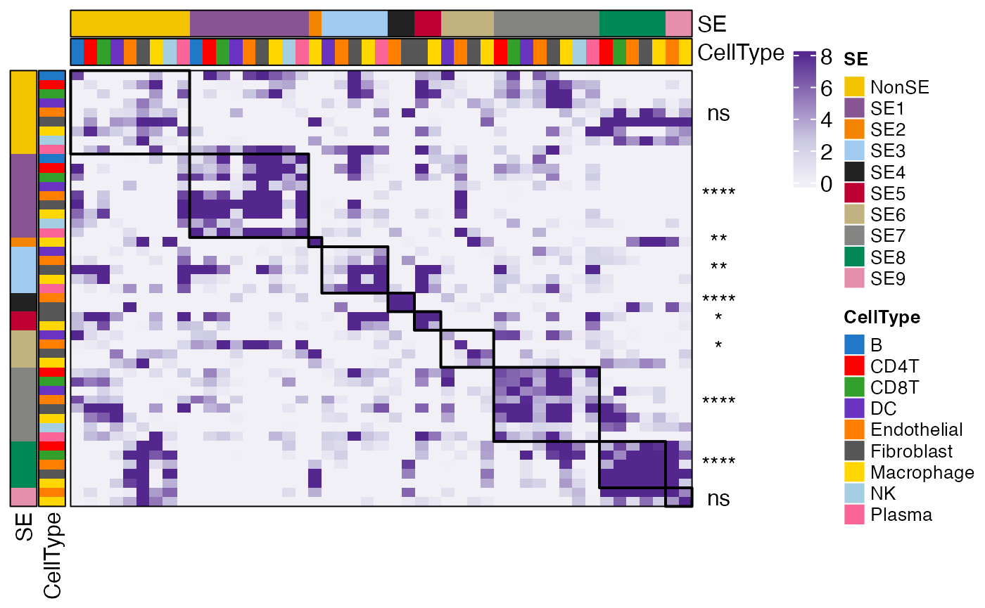
Here, in this small demo data, we can see strong colocalization of cell states within most SEs, whereas SE9 shows a weaker pattern, although it approaches statistical significance (P < 0.1). In contrast, the NonSE group, serving as a negative control, does not exhibit spatial colocalization.
Validation: spatial autocorrelation
Users can also validate the SEs by assessing the spatial autocorrelation with Moran’s I. To control for bias, permutation experiments will be performed to normalize Moran’s I into z-scores using the ComputeNormalizedMoranI function.
## For quick test run, test with 10 permutations were performed.
morani_zscore = ComputeNormalizedMoranI(scmeta, coords = c("X", "Y"),
                                        SE = "SE", CellType = "CellType",
                                        nperm = 10, ncores = 8)
morani_zscore
## NonSE SE1 SE2 SE3 SE4 SE5 SE6 SE7
## 12.71255 106.88797 34.95432 24.53143 110.12950 13.09989 14.99281 23.38682
## SE8 SE9
## 83.04186 10.32977Validation: average expression of SE markers
Users can also validate the SEs by visualizing the average expression of SE consensus markers across recovered SEs using the AverageMarkerExpression function.
## The function is built on Seurat functions, so first create a Seurat object.
obj = CreateSeuratObject(scdata, meta.data = scmeta)
obj = NormalizeData(obj)
By default, the AverageMarkerExpression function compute the average expression of SE consensus markers from Zhang et al., Nature 2026 paper.
## Visualize average expression of SE consensus markers across recovered SEs
res = AverageMarkerExpression(obj, group.by = "SE")
plot(res$p)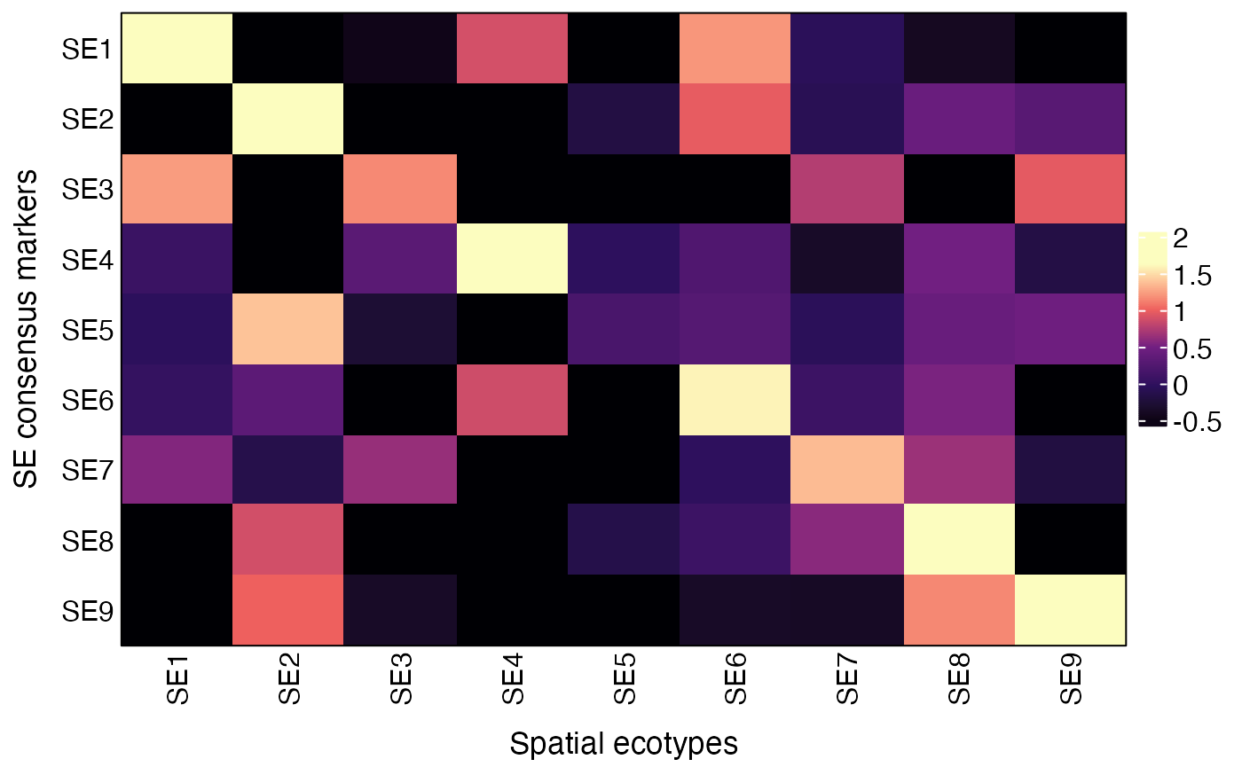
# Underlying data
res$AvgExp
## SE1 SE2 SE3 SE4 SE5 SE6
## SE1 1.63899149 -0.7067854 -0.4808280 0.8900028 -1.07180027 1.21067361
## SE2 -0.84198747 1.7084204 -0.6388041 -1.6401970 -0.19640606 0.97722401
## SE3 1.23530812 -1.2044554 1.1599992 -0.5802536 -0.84596171 -0.85957318
## SE4 0.06104092 -2.1637758 0.3105004 1.6581537 -0.03363019 0.23035569
## SE5 -0.04421435 1.3939729 -0.2878237 -2.3379710 0.17834575 0.27247684
## SE6 0.01721607 0.3289262 -0.8663956 0.8662647 -0.86950581 1.59766483
## SE7 0.55549363 -0.1465396 0.6349276 -2.1011003 -0.72279879 -0.03098458
## SE8 -1.22153700 0.8819891 -0.6609707 -0.6608298 -0.15405488 0.07337827
## SE9 -1.02337627 1.0094264 -0.3752031 -0.6409218 -1.01265650 -0.37474314
## SE7 SE8 SE9
## SE1 -0.06272876 -0.4191507 -0.9983748
## SE2 -0.09267733 0.4311746 0.2932529
## SE3 0.75394104 -0.6232041 0.9641996
## SE4 -0.37194620 0.4923575 -0.1830561
## SE5 -0.06336877 0.4210737 0.4675086
## SE6 0.07290969 0.5261576 -1.6732377
## SE7 1.36375460 0.6531338 -0.2058864
## SE8 0.58219283 1.9611643 -0.8013322
## SE9 -0.38983885 1.1548420 1.6524713The AverageMarkerExpression
function can also be used to visualize the average expression of
user-defined gene sets by specifying the markers parameter
as a list of gene lists.
genesets = list(set1 = c("FOS", "EGR1", "DUSP1", "JUNB", "JUN", "FOSB"),
                set2 = c("SPP1", "CCL2", "MMP9"),
                set3 = c("CXCL12", "TGFBR2", "PDK4", "HLA-DMA"),
                set4 = c("ACTA2", "CAV1", "CLDN5"),
                set5 = c("LRP1", "MAFB"),
                set6 = c("CXCL2", "NFKBIA", "CDKN1A"),
                set7 = c("STAT1", "TAP1", "HLA-A", "HLA-B", "HLA-C", "B2M"),
                set8 = c("PKM", "PCNA", "BST2"),
                set9 = c("NRP1", "ITGB1", "CD276"))
res = AverageMarkerExpression(obj, group.by = "SE", genesets = genesets)
plot(res$p)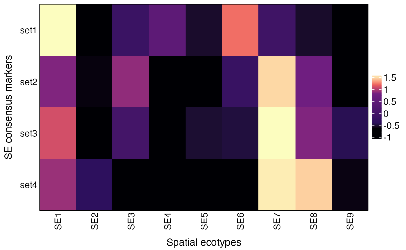
Session info
The session info allows users to replicate the exact environment and identify potential discrepancies in package versions or configurations that might be causing problems.
## R version 4.4.1 (2024-06-14)
## Platform: aarch64-apple-darwin20
## Running under: macOS 26.4.1
##
## Matrix products: default
## BLAS:   /Library/Frameworks/R.framework/Versions/4.4-arm64/Resources/lib/libRblas.0.dylib
## LAPACK: /Library/Frameworks/R.framework/Versions/4.4-arm64/Resources/lib/libRlapack.dylib;  LAPACK version 3.12.0
##
## locale:
## [1] en_US.UTF-8/en_US.UTF-8/en_US.UTF-8/C/en_US.UTF-8/en_US.UTF-8
##
## time zone: America/Los_Angeles
## tzcode source: internal
##
## attached base packages:
## [1] parallel  stats     graphics  grDevices utils     datasets  methods
## [8] base
##
## other attached packages:
##  [1] pals_1.9              SpatialEcoTyper_1.0.3 NMF_0.28
##  [4] Biobase_2.64.0        BiocGenerics_0.50.0   cluster_2.1.6
##  [7] rngtools_1.5.2        registry_0.5-1        RANN_2.6.2
## [10] Matrix_1.7-0          data.table_1.16.0     Seurat_5.1.0
## [13] SeuratObject_5.0.2    sp_2.1-4              ggplot2_3.5.1
## [16] dplyr_1.1.4
##
## loaded via a namespace (and not attached):
##   [1] RcppAnnoy_0.0.22       splines_4.4.1          later_1.3.2
##   [4] R.oo_1.26.0            tibble_3.2.1           polyclip_1.10-7
##   [7] fastDummies_1.7.4      lifecycle_1.0.4        sf_1.1-0
##  [10] doParallel_1.0.17      globals_0.16.3         lattice_0.22-6
##  [13] MASS_7.3-60.2          magrittr_2.0.3         plotly_4.10.4
##  [16] sass_0.4.9             rmarkdown_2.28         jquerylib_0.1.4
##  [19] yaml_2.3.10            httpuv_1.6.15          sctransform_0.4.1
##  [22] spam_2.10-0            spatstat.sparse_3.1-0  reticulate_1.39.0
##  [25] mapproj_1.2.11         cowplot_1.1.3          pbapply_1.7-2
##  [28] DBI_1.3.0              RColorBrewer_1.1-3     maps_3.4.2
##  [31] abind_1.4-5            Rtsne_0.17             R.utils_2.12.3
##  [34] purrr_1.0.2            circlize_0.4.16        IRanges_2.38.1
##  [37] S4Vectors_0.42.1       ggrepel_0.9.6          irlba_2.3.5.1
##  [40] listenv_0.9.1          spatstat.utils_3.1-0   units_1.0-1
##  [43] goftest_1.2-3          RSpectra_0.16-2        spatstat.random_3.3-1
##  [46] fitdistrplus_1.2-1     parallelly_1.38.0      pkgdown_2.1.0
##  [49] leiden_0.4.3.1         codetools_0.2-20       tidyselect_1.2.1
##  [52] shape_1.4.6.1          matrixStats_1.4.1      stats4_4.4.1
##  [55] spatstat.explore_3.3-2 jsonlite_1.8.8         GetoptLong_1.0.5
##  [58] e1071_1.7-16           progressr_0.14.0       ggridges_0.5.6
##  [61] survival_3.6-4         iterators_1.0.14       systemfonts_1.1.0
##  [64] foreach_1.5.2          tools_4.4.1            ragg_1.3.2
##  [67] ica_1.0-3              Rcpp_1.0.13            glue_1.7.0
##  [70] gridExtra_2.3          xfun_0.52              withr_3.0.1
##  [73] BiocManager_1.30.25    fastmap_1.2.0          boot_1.3-30
##  [76] fansi_1.0.6            spData_2.3.4           digest_0.6.37
##  [79] R6_2.5.1               mime_0.12              wk_0.9.5
##  [82] textshaping_0.4.0      colorspace_2.1-1       scattermore_1.2
##  [85] tensor_1.5             dichromat_2.0-0.1      spatstat.data_3.1-2
##  [88] R.methodsS3_1.8.2      utf8_1.2.4             tidyr_1.3.1
##  [91] generics_0.1.3         class_7.3-22           httr_1.4.7
##  [94] htmlwidgets_1.6.4      spdep_1.4-2            uwot_0.2.2
##  [97] pkgconfig_2.0.3        gtable_0.3.5           ComplexHeatmap_2.20.0
## [100] lmtest_0.9-40          htmltools_0.5.8.1      dotCall64_1.1-1
## [103] clue_0.3-65            scales_1.3.0           png_0.1-8
## [106] spatstat.univar_3.0-1  knitr_1.48             rstudioapi_0.16.0
## [109] reshape2_1.4.4         rjson_0.2.22           nlme_3.1-164
## [112] proxy_0.4-27           cachem_1.1.0           zoo_1.8-12
## [115] GlobalOptions_0.1.2    stringr_1.5.1          KernSmooth_2.23-24
## [118] miniUI_0.1.1.1         s2_1.1.9               desc_1.4.3
## [121] pillar_1.9.0           grid_4.4.1             vctrs_0.6.5
## [124] promises_1.3.0         xtable_1.8-4           evaluate_0.24.0
## [127] magick_2.8.5           cli_3.6.3              compiler_4.4.1
## [130] rlang_1.1.4            crayon_1.5.3           future.apply_1.11.2
## [133] classInt_0.4-11        plyr_1.8.9             fs_1.6.4
## [136] stringi_1.8.4          viridisLite_0.4.2      deldir_2.0-4
## [139] gridBase_0.4-7         munsell_0.5.1          lazyeval_0.2.2
## [142] spatstat.geom_3.3-2    RcppHNSW_0.6.0         patchwork_1.2.0
## [145] future_1.34.0          shiny_1.9.1            highr_0.11
## [148] ROCR_1.0-11            igraph_2.0.3           bslib_0.8.0